I Trained a Chess Model on Just $14
I recently created my own hybrid-transformer model trained specifically to plan implicitly rather than explicitly, called the Liquid Chess Model.
The model and its weights are available at MostLime/lcm-chess with a playable chess interface at MostLime/lcm-chess-playground.
What is this?
Unlike most chess bots, this one is based off of a language model’s architecture. The backbone of the model comes from Liquid AI’s LFM2, a highly efficient hybrid transformer architecture that is both faster and stronger than its standard attention counterparts. This makes LCM blazingly fast during use.
The LFM2 architecture is made up of two types of blocks:
- 6 GQA (Grouped-Query-Attention) blocks, the standard attention block for LLMs
- 10 LIV (Linear Input-Varying) convolution blocks
The LIV blocks in particular are the highlight of the architecture, as unlike GQA which expands with quadratic complexity as context length increases, LIV expands with linear complexity and requires less RAM. This makes the LFM2 model family very efficient.
For those who want a more technical or in-depth explanation for how LFM2 or LIV convolution blocks work, LFM2’s technical report from Liquid AI is a great read.
My modifications
Since LFM2’s release, several notable training and architectural enhancements have been discovered. Because I love learning about new tech, I chose to incorporate these upgrades into the model:
Token Order Prediction
Token Order Prediction, or TOP, essentially teaches the model to plan implicitly and is the main reason why I began this project. Token Order Prediction is a training method, meaning it’s not part of the model itself but rather the algorithm used to train it. Unlike standard next-token prediction (where the model has to predict the next token in the sequence and is tuned based on its output), TOP provides every future token in the sequence and asks the model how ‘close’ each token is to the current token. This additional training auxiliary teaches the model chess game structure and planning.
For instance, with the sequence ‘never gonna’ NTP would only try to correctly predict the next token, in this case ‘give’. However, TOP would be given all future tokens: ‘give’, ‘you’, and ‘up’ and for each future token, the model is asked how close that token to the current token in the sequence, and the model is tuned to provide the correct order. The following diagram from TOP’s paper might help.

Token order prediction essentially teaches the model how to predict future tokens ahead of time within its own internal structure. While TOP had mainly been tested on language modeling tasks, when reading the paper I immediately thought: this could be used for chess.
Chess is inherently a game of planning. Humans plan, even bots plan. But planning takes time, and time is expensive. What if the model was taught to plan within its own weights, without any explicit thinking? The top human chess players already do this in bullet or blitz chess. The model would be able to answer instantly without any reliance on explicit search algorithms like Monte Carlo Tree Search.
TOP, I thought, could solve that problem. It teaches the model to predict where tokens might be in the future, providing a clearer signal for future-move prediction than NTP. But when I looked for models that use this method, there were none. TOP was released in mid 2025 so no transformer-based models had the chance to even try it. I would be the first.
TOP isn’t a replacement to NTP, but rather an addition to it. Before the main training run, I performed a variety of ablations on several configurations. I tested a variety of different mixes of TOP and NTP, some where NTP is weighed more than TOP and vice versa. After all these ablations, I confirmed three things:
- TOP does help the model learn how to play better chess.
- Placing more weight on TOP is better than placing more weight on NTP
- The optimal balance of TOP:NTP weight is 70:30
The optimal TOP:NTP weight being 70:30 was a good sign. In the results in my small-scale ablations, I noticed that pure NTP had a loss of around 3.4, while the 70:30 ratio of TOP to NTP has a loss of around 3.2. TOP and NTP combined was clearly much better than NTP alone. These were small-scale ablations, so the true optimal ratio is unknown and I do not know how the convergence behaviour might be in larger scale runs.
The Muon Optimizer
Despite being a relatively new optimizer, Muon sweeps the floor with AdamW, which has been standard for several years now.
The Muon Optimizer, introduced by Keller Jordan and scaled by Moonshot AI is more efficient, effective, and stable than AdamW. The following image from Keller Jordan’s blog post illustrates this claim.
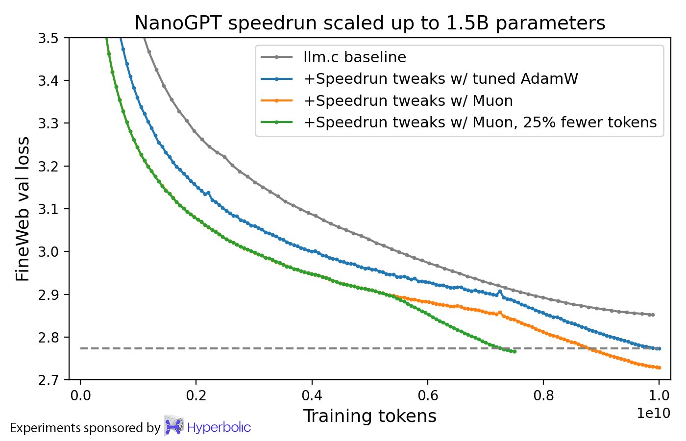
As time progresses, more and more labs use Muon as a replacement for AdamW, most notable of which are Moonshot AI’s Kimi K2 and Z.ai’s GLM-4.5.
Learnable Multipliers
Learnable Multipliers, or LRMs, allow the model to tune the magnitude of its own layers during training. This is a simple upgrade, but was discovered fairly recently in January 2026 by Velikanov et al.
There is no noticable downside to LRMs, and they appear to be a ‘free upgrade’. To make sure, I tested a couple ablations and it appeared not to make the model much better or worse. The research done on LRMs seem to suggest that they become useful much later in training. So, I assumed that the benefit of LRMs will become more obvious in the main training run.
FlashAttention-4
Like TOP & Muon, this is a training modification. FlashAttention-4 was released literally the day I began training and since I was using a B200 to train the model, I thought “why not try FlashAttention-4, maybe it’ll save me some credits?”
While it worked, several large loss spikes appeared during training that seemed abnormal. The reason for those loss spikes isn’t completely evident, though I speculate it may have been due to bugs in the implementation of FlashAttention-4. The loss graph can be seen later in the blog post near the end of the section about the main training run.
Generating the dataset
To train LCM, I generated two datasets ahead of time:
Dataset one: 7.8M of the highest-elo Lichess games
Dataset two: 7.8M of the highest-elo Lichess games + 100k highly-rated OTB (or outside of Lichess) games from The Week in Chess
I published the first dataset on Hugging Face. However upon emailing the author of TWIC, I was denied the permission to distribute his games publicly. For this reason, the second dataset is private.
For ease-of-access, I trained on my public dataset for each of my ablation runs. The main training run used the private dataset because of how much higher quality it is.
You can find specifics about the public dataset on the Hugging Face page. To create it, I crawled the entirety of the Lichess Elite database and processed it by:
- keeping only the highest-elo games
- making sure that a large portion of games end in checkmate (to avoid noisy training data)
- keeping only drawed games that are forced and removing games ending in timeout
- tokenizing the dataset and generating an NTP mask (to only train the model on the winning side)
And the TWIC database was crawled likewise.
The average elo of the datasets are 2600, and the tokenizer’s vocabulary contains every single legal chess move, as well as a handful of additional tokens (terminal tokens, POV token, and a padding token).
While almost every other chess model in history is trained only on positions, we train the model on the full game history. This limits the model, since it wouldn’t be able to solve puzzles or work in any context where only the board position is given. However, training on the full game history is necessary because TOP predicts the order of future tokens, and we can’t do that without the full sequence. I will attempt to solve this problem in future work.
The ablations
The ablations were done on Kaggle using an Nvidia P100 GPU. I trained the 29M parameter model on 50,000 games from my public Lichess-based dataset across one epoch with a batch size of 64. I tested various configurations such as:
- with/without LRM (with LRM won)
- 8 vs 16 layers (16 layers won)
- ratio of GQA blocks to LIV blocks (6:10 won)
- loss weight of TOP to NTP (70:30 won)
- several other minor configurations
all done in search of the lowest NTP loss. The reason why we don’t take into account the combined loss is because accuracy in predicting the next move is the goal here, and TOP is only a way to increase that accuracy.
The ablations were done with the knowledge that they are not a completely accurate representation of the final run, as 50,000 games is not nearly enough to record the model’s ability to converge. Luckily, most of the default configurations performed best (aside from the TOP to NTP weight ratio, whose default is 50:50).
The main training run
The main training run uses the optimal configurations found during ablations and extends our training from 50,000 games in one epoch to 7.9M games from my private dataset across 3 epochs with a batch size of 2048. We use Modal as our GPU provider, using a B200.
Modal was picked because they provided great GPUs and $30 of free credits per month. The free credits were essential, because I am a high-school student with no source of income.
Using a B200 might seem excessive or expensive to some, but B200s are some of the cheapest GPUs to rent because they train models extraordinarily fast. B200s are more expensive per-hour, but they are typically worth it because they train much faster, and therefore incur fewer billed hours. Moreover, using larger batch sizes and tuning the hyperparameters allows you to utilize more of the GPU, lowering costs more. This is how I saved lots of credits during training.
The training run completed in 1hr 30min, costing $14.63 to train ($14.17 for the B200 and the rest for CPU and memory usage). The following is the loss graph of the model across the 11k steps it was trained on, with the y-axis being loss in logarithmic scale.
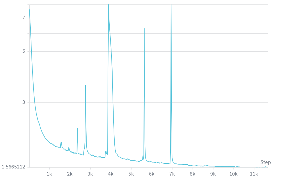
The loss plateaued to around 1.56. While it is unknown why there are so many large loss spikes, I suspect it is due to FlashAttention-4 being so recent. While some of the loss spikes occured at the ends and starts of some of the epochs, the last epoch notably had no spike at all. The fact that the third epoch does not have any loss spike at all is interesting and weird.
Model quality
Quantitative evaluations
My first method of evaluation was against Stockfish’s skill levels. Stockfish, while normally super-human, allows you to reduce its elo with a ‘skill level’ parameter. Stockfish provides skill levels 0-20, going from roughly 1350 elo to 3170 elo. To test the model, I ran several hundred games against various levels of Stockfish. While results were noisy, my model performs around on-par (or slightly worse) than level 0, performing around 1250-1400 elo.
My second method of evaluation was by pre-generating 5,000 Stockfish self-play games (in which one player was maximum-level Stockfish and the other player was a randomly chosen Stockfish skill level) and directly compared my model’s responses to Stockfish’s responses. This precisely measures how many of our model’s moves are ‘best moves’.
In the evaluation, my model has a top-1 accuracy (how well the model responds with Stockfish’s most prefered move) of around 30% and a top-3 accuracy (a more important metric given that most positions have several ‘best moves’) of around 50%. This is a surprisingly great result, given that most moves outside of this range are still good or excellent moves.
While the first method provides an elo, it’s rather noisy. Often, the model will have a 30% win-rate against 1350-rated Stockfish, and often it will have a 50% win-rate. Moreover, it will occasionally win against some of the highest rated bots (~2500 elo in the evaluation). The reason for the latter issue will be discussed later.
The second method is far more precise, but blunders do not impact the result as much as it should.
Qualitative evaluations
I analyzed the model’s performance against myself, bots, and other humans. The model has great opening knowledge, which is expected for something trained on 7.9M of the best games. Moreover, most of the moves it plays are good moves or better, and it may often play well against strong players. However, the reason for the low elo rating observed earlier is due to one fatal flaw: the bot is blind.
For some unknown reason, the model will make one or two disastrous blunders per game. These are illogical, highly obvious blunders. Most often, it will ignore a piece the opponent is hanging. It will also occasionally hang its own pieces in illogical ways by leaving them completely undefended, or hang a mate in one. This problem happens often enough for the model to lose most games against competent players.
Why it plays like this
While the true reason is unknown, I highly believe it’s a fault of poor data. The dataset only contains games of very high-elo players (~2600 elo) and at that level, almost nobody hangs pieces or mate-in-ones. Moreover, given that each player knows that the other player wouldn’t hang pieces or mate-in-ones, neither side attempts any ‘simple’ threats. Because of the lack of data, the model never learns how to properly respond when the opponent hangs a rook, and doesn’t notice obvious mate-in-ones because they never appear in the data. The model becomes blind against certain moves.
A second theory is that the lack of board state provided to the model forces the model to reconstruct the board state. This can use up some of the capacity in the lower layers of the model, limiting its reasoning capacity. Moreover, it could also lead to gaps in the model’s reconstructed board state, leading it ‘forgetting’ or ‘missing’ certain moves that would be obvious to others. This is like having to play chess blindfolded rather than being able to see the actual board. You must rely on your memory alone.
It is impossible to tell which theory is the reason for our problems, or even if both theories are the root cause.
What I tried to do to fix it
To fix this, I spent three days straight with no break and spent over 30 hours in the hopes that I might find a solution. I tried various methods, for example I:
- collected thousands of self-play games, analyzed them for blunders, and performed soft-target SFT on the model on those blunders, fixed with Stockfish
- distilled Stockfish (against a variety of Stockfish levels) into the model
- performed RL on the model
And while it doesn’t look like much by itself, it is important to note that I tested several variations of each method. For example, the soft-target SFT on blunders had several variations where I:
- Didn’t use soft-target
- Shifted what counted as a ‘blunder’
- Changed hyperparameters
- Used various methods to keep the model from forgetting its chess knowledge catastrophically
and many other changes.
However, every single method either regressed or was on-par with the base model on the quantitative evaluations, and was always worse on the qualitative evaluations. None of the methods worked.
Future work
In my eyes, this model is a failure. But failures are inevitable in this line of work and we should instead strive to learn the most from failures. The only way to learn from failures is to try to correct them. I intend to create a v2 LCM model soon, likely next month when my Modal credits refresh, with these changes:
- An improved data pipeline: I may choose to go down the path of Allie, where an elo token is prepended to the games and we’d be able to train on a variety of elo ranges on a larger dataset. This may avoid disastrous issues like simple blunders, but takes us off the path off creating the best transformer-based chess model. Additionally, there exists a giant lc0 self-play dataset that I intend to include. This lc0 dataset likely has far higher quality moves than my current dataset, as lc0 has an elo above any human.
- More in-depth ablations: It feels dumb not to have done this earlier, but I definitely need to perform more in-depth ablations with the model architecture. For example, I need to know whether or not our hybrid transformer architecture is actually better than a regular transformer architecture.
- A re-designed architecture: It is clear that many of the problems here come from a flawed architecture. I intend to experiment on the idea of providing the current board state alongside Stockfish-generated future moves from that position onwards. This should provide the benefits of a board state alongside the benefits of token order prediction.
- Some FlashAttention-4 experiments: I am still unsure how the loss spikes were so crazy during training, so I’d like to investigate FlashAttention-4 in case it might be the culprit. Hopefully FlashAttention-4 will have had these potential issues fixed by then, if it is the culprit.
Links
- Model’s Hugging Face page: Mostlime/lcm-chess
- Play against the model yourself: Mostlime/lcm-chess-playground
- Dataset’s Hugging Face page: Mostlime/chess-elite-uci
References
- LFM2 blog page: Liquid.ai
- LFM2 technical report: arXiv
- Token order prediction paper: arXiv
- Learnable Multipliers paper: arXiv
- Muon Optimizer: Keller Jordan blog